Processing and Using SafeGraph Stay-at-Home Data
distancing_vignette.Rmd
library(SafeGraphR)This vignette will walk you through the process of reading in, processing, and displaying SafeGraph stay-at-home data.
Note that the stay-at-home-data is no longer being updated as of April 19, 2021. However, this should work for the old data.
This vignette will work with data from the social-distancing/v2/ SafeGraph Amazon Web Services bucket (see the SafeGraph Catalog for more information), which is no longer available.
Note that throughout this vignette, we will be working with data manipulation using the data.table package. data.table is used throughout SafeGraphR (and on the backend) because it is very fast and can handle large data sets easily. However, once the data is read in and processed, it’s often no longer necessary to use data.table if you prefer something else. The code in this vignette could have easily used, for example, dplyr instead. If you are having trouble understanding the code chunks because you’re familiar with dplyr but not data.table, see this guide that links the two.
Reading in Data
We will read in the distancing data using the read_distancing() function. This relies on the files in the social-distancing/v2 bucket in the Amazon Web Services bucket, which you can download using safegraph_aws() (or using the AWS CLI). See the SafeGraph Catalog.
Once we’ve downloaded it, the files will be in a YEAR/MONTH/DAY/FILE structure. We can tell it where to begin and end reading files (we probably don’t want ALL the files - that would be very large!) by specifying a start and end date. Let’s get all the data from June 1 to June 14, 2020.
IMPORTANT: by default, read_distancing() will only select the variables necessary to get stay-at-home percentages, and will aggregate by the state and county level. If you want more variables from the data, change select. And if you want the original raw census block group-level data (origin_census_block_group), change by. There is also an option to filter the data.
# Our working directory is in the same folder as the "2020" folder
distancing <- read_distancing(
   start = lubridate::ymd('2020-06-01'),
   end = lubridate::ymd('2020-06-14')
)
data(distancing)
distancing[]
#>        state_fips county_fips device_count completely_home_device_count
#>     1:         01         053         2735                          704
#>     2:         01         073        55056                        15661
#>     3:         01         089        30082                         9208
#>     4:         01         095         8557                         2147
#>     5:         01         097        32792                         9484
#>    ---
#> 45154:         35         021           42                            8
#> 45155:         32         009           61                           17
#> 45156:         48         433          137                           35
#> 45157:         48         359          211                           44
#> 45158:         31         171           52                            9
#>        part_time_work_behavior_devices full_time_work_behavior_devices
#>     1:                             169                              38
#>     2:                            2818                             792
#>     3:                            1510                             331
#>     4:                             520                              94
#>     5:                            1912                             461
#>    ---
#> 45154:                               3                               1
#> 45155:                               2                               2
#> 45156:                              11                               4
#> 45157:                              25                               3
#> 45158:                               1                               1
#>              date
#>     1: 2020-06-14
#>     2: 2020-06-14
#>     3: 2020-06-14
#>     4: 2020-06-14
#>     5: 2020-06-14
#>    ---
#> 45154: 2020-06-01
#> 45155: 2020-06-01
#> 45156: 2020-06-01
#> 45157: 2020-06-01
#> 45158: 2020-06-01
Processing Data
We will be calculating and using the percentage of each county that is staying home, which is completely_home_device_count/device_count, but we may need to do some adjustments.
We have a few goals at this point:
- Do any further aggregation or adjustments we like
- Smoothe out weekend effects
- Make the data presentable!
1. Do any further aggregation or adjustments we like
Any additional adjustments that we do depend on the level we want the eventual data at. If we want to aggregate the data up to a higher level (perhaps to get stay-at-home by state), we might want to do sample_size_adjust() to account for different sampling rates across regions. See the Patterns Vignette for an example of using sample_size_adjust().
If instead we want to report the granular individual-level data, we should perform Bayesian shrinkage with hb_shrink(). so that we don’t get strange results from small regions with few people in them.
Hierarchical Bayesian shrinkage basically says “we’re going to start by assuming that you, the individual county, are exactly the same as the overall state. Then we adjust that assumption by looking at your individual data. If you’re small, we won’t adjust much, since we don’t see much from you. But if you’re big, we adjust a lot.” We will be doing this to shrink counties to states, but you could instead shrink census block groups to counties or states.
hb_shrink() is a shrinkage function that only works with proportions. Conveniently, “the proportion staying home” is a proportion! Note, by the way, that if we had CBG-level data but wanted the eventual data at the county level, shrunk to the state level, we would sum up completely_home_device_count and device_count to the county level before using hb_shrink().
distancing <- distancing[,.(county_fips = county_fips,
                            completely_home_device_count = completely_home_device_count,
                            device_count = device_count,
                            raw_stay_home = completely_home_device_count/device_count,
                            shrunk_stay_home = hb_shrink(completely_home_device_count,device_count)),
                         by = .(state_fips, date)]
distancing[]
#>        state_fips       date county_fips completely_home_device_count
#>     1:         01 2020-06-14         053                          704
#>     2:         01 2020-06-14         073                        15661
#>     3:         01 2020-06-14         089                         9208
#>     4:         01 2020-06-14         095                         2147
#>     5:         01 2020-06-14         097                         9484
#>    ---
#> 45154:         78 2020-06-01         010                          433
#> 45155:         78 2020-06-01         030                          381
#> 45156:         78 2020-06-01         020                           27
#> 45157:         69 2020-06-01         110                           36
#> 45158:         69 2020-06-01         120                            6
#>        device_count raw_stay_home shrunk_stay_home
#>     1:         2735     0.2574040        0.2567292
#>     2:        55056     0.2844558        0.2843217
#>     3:        30082     0.3060967        0.3057083
#>     4:         8557     0.2509057        0.2508285
#>     5:        32792     0.2892169        0.2889632
#>    ---
#> 45154:         1125     0.3848889        0.3832164
#> 45155:         1055     0.3611374        0.3600957
#> 45156:          114     0.2368421        0.2576238
#> 45157:          109     0.3302752        0.3432126
#> 45158:           13     0.4615385        0.4173651
2. Smooth out weekend effects and scale
Next we will likely want to smooth things out and handle day-of-week effects by using the ma() moving average function. Don’t forget to sort first!
# Not actually run since we only have 14 days of data here anyway
data.table::setorder(distancing, state_fips, county_fips, date)
distancing[, shrunk_stay_home := ma(shrunk_stay_home), by = c('state_fips', 'county_fips')]
Now we may want to consider scaling the data relative to a specific date in the past. This isn’t as necessary for distancing data as it is for patterns data, but it can make things easier to compare sometimes.
We’ll skip this scale-to-a-certain-date step with our example (see the Patterns Vignetter for an example of how this is done), but I will provide some code for doing a year-on-year adjustment, in case you want to combine multiple years of data to see how much more at-home we are this year than last year.
# let's pretend we have another year by just duplicating the data we have
fake_lastyear <- data.table::copy(distancing)
fake_lastyear[,date := date - lubridate::years(1)]
fake_lastyear[,shrunk_stay_home := shrunk_stay_home - runif(45158, max = .02)]
fake_lastyear <- rbind(distancing, fake_lastyear)
fake_lastyear_scaled <- scale_yoy(fake_lastyear,
yoy_vars = 'shrunk_stay_home',
by = c('state_fips','county_fips'))
# Notice the "2019" data has no growth since we din't give it 2018 data to grow from
fake_lastyear_scaled[,c('date','state_fips','county_fips','shrunk_stay_home','shrunk_stay_home_lag','shrunk_stay_home_YOY')]
#> date state_fips county_fips shrunk_stay_home shrunk_stay_home_lag
#> 1: 2019-06-01 01 001 0.2225649 NA
#> 2: 2019-06-02 01 001 0.2199512 NA
#> 3: 2019-06-03 01 001 0.1865503 NA
#> 4: 2019-06-04 01 001 0.1976422 NA
#> 5: 2019-06-05 01 001 0.1932117 NA
#> ---
#> 90312: 2020-06-10 78 030 0.2962983 0.2785883
#> 90313: 2020-06-11 78 030 0.2995778 0.2821803
#> 90314: 2020-06-12 78 030 0.2693960 0.2683497
#> 90315: 2020-06-13 78 030 0.3269283 0.3210544
#> 90316: 2020-06-14 78 030 0.3441301 0.3410606
#> shrunk_stay_home_YOY
#> 1: NA
#> 2: NA
#> 3: NA
#> 4: NA
#> 5: NA
#> ---
#> 90312: 0.063570791
#> 90313: 0.061654063
#> 90314: 0.003899023
#> 90315: 0.018295575
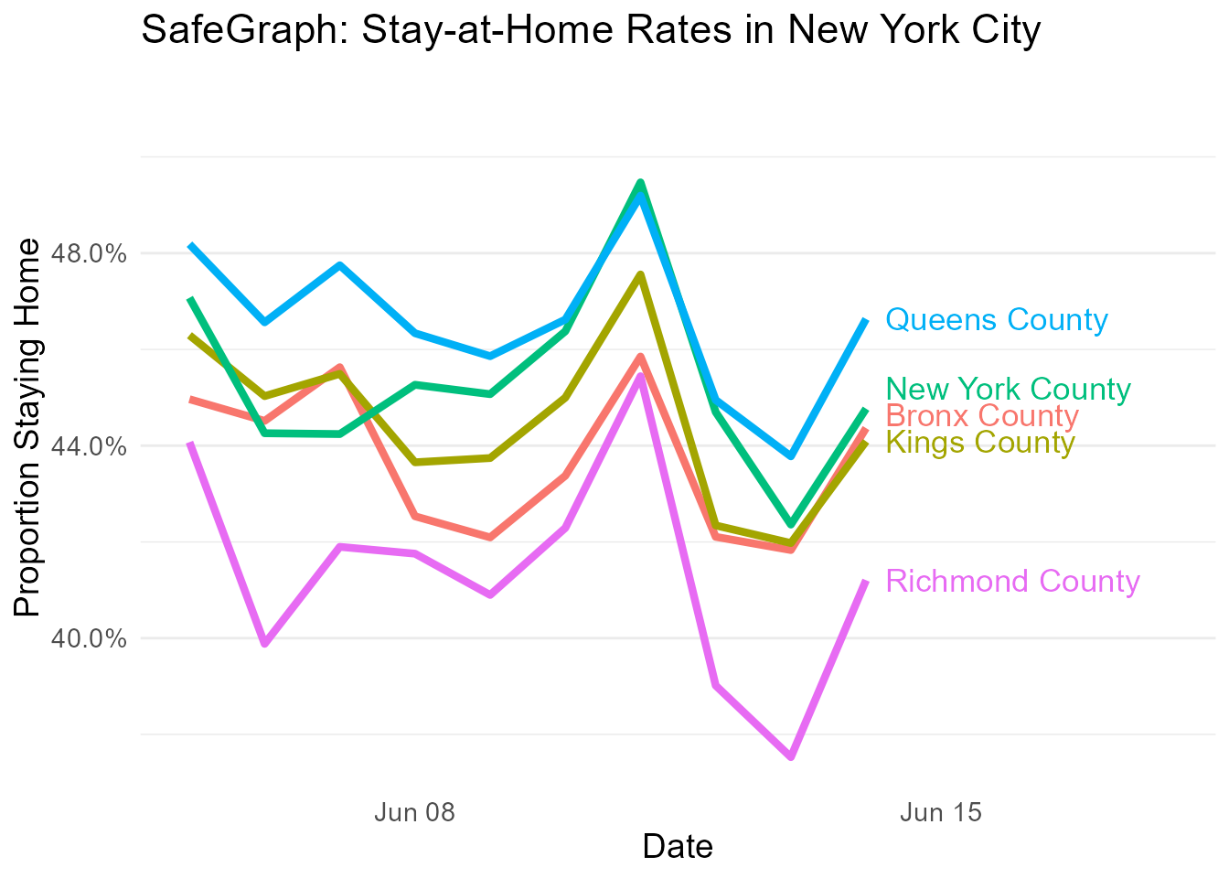
#> 90316: 0.0089998343. Make the data presentable!
Let’s bring in the state and county names for nice labeling
Let’s take a look at the five boroughs of New York!
distancing[statename == 'New York' &
             countyname %in% paste(c('New York',
                              'Kings',
                              'Queens',
                              'Bronx',
                              'Richmond'),'County')] %>%
  ggplot2::ggplot(ggplot2::aes(x = date, y = shrunk_stay_home, color = countyname, label = countyname)) +
  ggplot2::geom_line(size = 1.5) +
  directlabels::geom_dl(ggplot2::aes(x = date + .25), method = list('last.bumpup', cex = 1.1)) +
  ggplot2::scale_y_continuous(labels = scales::percent) +
  ggplot2::scale_x_date(limits = c(min(distancing$date) + 4,max(distancing$date) + 4)) +
  ggplot2::guides(color = 'none') +
  ggplot2::theme_minimal() +
  ggplot2::labs(x = "Date", y = "Proportion Staying Home",
                title = "SafeGraph: Stay-at-Home Rates in New York City") +
  ggplot2::theme(panel.grid.major.x = ggplot2::element_blank(),
                 panel.grid.minor.x = ggplot2::element_blank(),
                 text = ggplot2::element_text(size = 14))
#> Warning: Removed 20 row(s) containing missing values (geom_path).
#> Warning: Removed 20 rows containing missing values (geom_dl).