Processing and Using SafeGraph Patterns Data
patterns_vignette.Rmd
library(SafeGraphR)This vignette will walk you through the process of reading in, processing, and displaying SafeGraph patterns data. This will look at the use of patterns data generally. For a more automated look at processing visits_by_day data for foot traffic over time, see the “Automatic Traffic-over-Time Processing” vignette.
This vignette will work with weekly data files, which could also be downloaded using safegraph_aws() if you have an AWS connection, or safegraph_api(). However, with only minor variation in the first section, the same processes could be applied to data downloaded from the SafeGraph shop, or to monthly patterns.
Note that throughout this vignette, we will be working with data manipulation using the data.table package. data.table is used throughout SafeGraphR (and on the backend) because it is very fast and can handle large data sets easily. However, once the data is read in and processed, it’s often no longer necessary to use data.table if you prefer something else. The code in this vignette could have easily used, for example, dplyr instead. If you are having trouble understanding the code chunks because you’re familiar with dplyr but not data.table, see this guide that links the two.
Reading in Data
We will be reading in data from the July 1, 2020 weekly patterns release (why only one week? To keep things small enough that the example data can be included in the package).
The read_patterns() function can read in a single patterns file. But most of the time you will probably be using read_many_patterns(), which reads multiple patterns files, processes them, and row-binds them together.
If you truly want the raw data, you are probably best off skipping read_many_patterns() and instead just doing list.files() %>% purrr::map(data.table::fread) %>% data.table::rbindlist(). However, this would return an enormous result, and you probably just want a subset of the data, or some aggregated data.
read_many_patterns() can perform multiple different aggregations in a single go, aggregating each of them across multiple files.
So how can we build a read_many_patterns() call? There are two main elements here: finding the files to read in, and then filling in the aggregation information in the by, fun, na.rm, filter, expand_int, expand_cat, and expand_name options.
For finding the files to fill in, you can use read_many_patterns() itself, if what you want is all the files you have downloaded. Just specify the dir and it will load all the .csv.gz files in the subfolders of that directory. Or, you can be more choosy about it! Use patterns_lookup() to generate a list of files (and, potentially, with a key and secret, download those files) that contain patterns information for a given set of dates (plus extra for moving-average purposes!). Then pass that filelist to the filelist option.
For aggregating, the by, fun, na.rm, filter, expand_int, expand_cat, and expand_name options are expanded further upon in read_patterns(). Effectively, they determine the level to aggregate the data to (data will be aggregated to the by-and-expanded-JSON-column-index level), the function to use for aggregation (fun), whether to only pull a subset of the data (filter), and which of the JSON columns in the data to expand before aggregating (expand_int OR expand_cat, with expand_name giving the name of the index variable to be created).
So for example, if we want to get the number of visits by day by NAICS code, we would want to set by = 'naics_code'. The visits-by-day variable is visits_by_day and is stored in the format [1,2,3,4,5,6,7] which can be extracted internally by expand_integer_json(), i.e. it’s a numeric JSON column (as opposed to a categorical JSON column like visits by CBG in the format {category: number, category: number} which can be extracted intenally by expand_cat_json()). So we set expand_int = 'visits_by_day'. When we do expand_int = 'visits_by_day', then expand_name will default to “day” so we don’t need to do anything there. We do want it to add up the visits by day across all the different POIs in that NAICS code, so fun = sum as default is fine. This gives us in total by = 'naics_code', expand_int = 'visits_by_day'.
# Not yet working code
patterns_naics_code <- read_many_patterns(by = 'naics_code', expand_int = 'visits_by_day')
Now instead let’s imagine we want the total number of all visits to any POI by county, but only in New York and New Jersey. Now we want to aggregate to the state/county level, so we want by = c('state_fips', 'county_fips') (don’t try just doing 'county_fips' as the same county FIPS code is reused across states). Again we want expand_int = 'visits_by_day'. However, now that we are looking just at New York and New Jersey, we need to use filter, which we can do by specifying the filter as a string. So filter = state_fips %in% c(34, 36), where 34 and 36 are the New Jersey and New York FIPS codes, respectively. So now we have by = c('state_fips', 'county_fips'), expand_int = 'visits_by_day', filter = 'state_fips %in% c(34, 36).
# Not yet working code
patterns_NY_NJ <- read_many_patterns(by = c('state_fips', 'county_fips'),
                                    expand_int = 'visits_by_day',
                                    filter = 'state_fips %in% c(34, 36)')
Those are the relevant aggregation options to follow. And, since we want both of them, we can get them both in one call (rather than having to read in the data separately for each, which is slow). We just toss each of these sets of options in a list(), adding the required option name to tell us which aggregation we’re doing, and then putting both of those lists in a bigger list() for multi.
# Not yet working code
patterns <- read_many_patterns(multi = list(
  list(name = 'patterns_naics',
       by = 'naics_code',
       expand_int = 'visits_by_day'),
  list(name = 'NY_NJ',
       by = c('state_fips', 'county_fips'),
       expand_int = 'visits_by_day',
       filter = 'state_fips %in% c(34, 36)')
))
What else do we need?
First, of course, we need to tell it where the patterns files are. We can specify dir (or it will just go to the working directory). Or if we want to do our own list.files() command and pick a subset, we can give it to filelist. Since we are working with new-format data that sits inside nested folders, we want to be sure to specify recursive = TRUE so as to look in those folders.
Second, if we want to aggregate (or filter) by NAICS code, which we do, we need to know the NAICS code of each POI. We can do that by processing the most recent monthly SafeGraph Core file using read_core. read_core will use the most recent Core file in the core_poi/ directory of the working directory - it will download the most recent one too if you give it an AWS key and secret! Then we can pass the resulting file to the naics_link option.
poi_link <- read_core(select = c('placekey','naics_code'))
# I probably at this point would save poi_link to disk - that took a while!
Next, if we want to use the state and county FIPS codes, we want to make sure that gen_fips = TRUE, which it is by default, so we’re good there. This uses fips_from_cbg() internally.
Fourth, patterns files don’t tell you what the first date in them is. read_many_patterns() will try to guess that date by the filepath. But if you want to be sure, you can set start_date for each of the files being read in. You can more easily find the starting dates using the find_date() function (which is what read_patterns() uses internally. Don’t forget to subtract lubridate::days(9) to get the starting date for non-backfill data!
Finally, and very important, if we are doing any sort of aggregation we probably want to specify select, a character vector of variables to be read in. If we don’t, then reading in the data will take way longer. Also, if some of those variables aren’t amenable to being aggregated with fun, you could get an error. We are planning to use the visits_by_day variable so we need that. We’ll also use poi_cbg (to be sent to fips_from_cbg() to get state_fips and county_fips), but that’s in by default whenever gen_fips = TRUE. We also need naics_code, but that isn’t read in from the file; rather it comes from the poi_link data we made. So we specify select = 'visits_by_day'.
See the SafeGraph docs for full documentation of all the available variables.
Note that select applies to the file as it’s read in before any aggregation, so it goes in read_many_patterns directly, not inside of multi.
In total, we have:
# Assume our working directory is the the /patterns/ folder
patterns <- read_many_patterns(recursive = TRUE,
                               naics_link = poi_link,
                               select = 'visits_by_day',
                               multi = list(
                                 list(name = 'patterns_naics',
                                      by = 'naics_code',
                                      expand_int = 'visits_by_day'),
                                 list(name = 'NY_NJ',
                                      by = c('state_fips', 'county_fips'),
                                      expand_int = 'visits_by_day',
                                      filter = 'state_fips %in% c(34, 36)')
))
Internally, this calls read_patterns() many times, followed by rbind_by_list_pos(). Then it re-aggregates across the multiple files it just read in (unless you set ).
The result will be patterns, a list, where patterns[[1]] (or patterns[['patterns_naics']]) contains the NAICS aggregation, and patterns[[2]] (or patterns[['NY_NJ']]) contains the New York/New Jersey aggregation. Let’s save those as their own objects (which will then be a part of the package so we can use real data in this vignette!).
# This data is one observation per NAICS code per day
pat_naics <- patterns[['patterns_naics']]
# This data is one observation per NY/NJ county per day
pat_NY_NJ <- patterns[['NY_NJ']]
# At this point I'd save both of these to disk, that took a whole five minutes!
rm(patterns)
# Now to load in for real!
data(pat_naics)
pat_naics[]
#>       naics_code state_fips county_fips visits_by_day day start_date       date
#>    1:         NA     105563      368142          9441   1 2020-06-22 2020-06-22
#>    2:         NA     105563      368142          9447   2 2020-06-22 2020-06-23
#>    3:         NA     105563      368142         10063   3 2020-06-22 2020-06-24
#>    4:         NA     105563      368142         10096   4 2020-06-22 2020-06-25
#>    5:         NA     105563      368142         10717   5 2020-06-22 2020-06-26
#>   ---
#> 9243:     928120        933        2663           147   3 2020-06-22 2020-06-24
#> 9244:     928120        933        2663           155   4 2020-06-22 2020-06-25
#> 9245:     928120        933        2663           152   5 2020-06-22 2020-06-26
#> 9246:     928120        933        2663            60   6 2020-06-22 2020-06-27
#> 9247:     928120        933        2663            40   7 2020-06-22 2020-06-28
data(pat_NY_NJ)
pat_NY_NJ[]
#>       state_fips county_fips naics_code visits_by_day day start_date       date
#>    1:         34          01         NA          5862   1 2020-06-22 2020-06-22
#>    2:         34          01         NA          5754   2 2020-06-22 2020-06-23
#>    3:         34          01         NA          5769   3 2020-06-22 2020-06-24
#>    4:         34          01         NA          5887   4 2020-06-22 2020-06-25
#>    5:         34          01         NA          6778   5 2020-06-22 2020-06-26
#>   ---
#> 2320:         36         123   40485879           253   3 2020-06-22 2020-06-24
#> 2321:         36         123   40485879           217   4 2020-06-22 2020-06-25
#> 2322:         36         123   40485879           294   5 2020-06-22 2020-06-26
#> 2323:         36         123   40485879           440   6 2020-06-22 2020-06-27
#> 2324:         36         123   40485879           245   7 2020-06-22 2020-06-28
Notice in looking at pat_naics that the missing-NAICS code POIs have been included. Also notice that state_fips and county_fips are nonsense. We loaded them in (for pat_NY_NJ) but then didn’t use them in aggregation! So it summed them up and they’re nonsense now. Same issue with naics_code in pat_NY_NJ. We can drop them.
pat_naics[,state_fips := NULL]
pat_naics[,county_fips := NULL]
pat_NY_NJ[,naics_code := NULL]
We will also need the normalization data to properly work with what we have. Normalization data is just in regular ol’ CSV files, so we can read everything in with read_many_csvs(). Since normalization files have year, month, and day columns, we can also set makedate = TRUE to get a date variable in there. If we only want to normalize at the national level, pick the ALL_STATES rows.
norm <- read_many_csvs(dir = "../normalization_stats/",
                       recursive = TRUE,
                       makedate = TRUE)[region == 'ALL_STATES']
norm[, region := NULL]
data(norm)
norm[]
#>    total_visits total_devices_seen total_home_visits total_home_visitors
#> 1:     50656915           17312070          23890767            14335375
#> 2:     50805493           16870682          23389482            14021137
#> 3:     52223098           17103600          23758844            14153853
#> 4:     52544946           17014972          23460878            13980621
#> 5:     54186679           16964900          23425016            13993356
#> 6:     49766561           16304498          22301353            13344340
#> 7:     45347171           16341487          23068199            13912816
#>          date
#> 1: 2020-06-22
#> 2: 2020-06-23
#> 3: 2020-06-24
#> 4: 2020-06-25
#> 5: 2020-06-26
#> 6: 2020-06-27
#> 7: 2020-06-28
Finally, if we want to do sample_size_adjust(), we will need the number of devices by region from the home panel summary files. We can also read this with read_many_csvs().
# Make sure that census_block_group is read as a character
# note colClasses is a data.table::fread() argument
panel <- read_many_csvs(dir = '../home_panel_summary',
                        colClasses = c(census_block_group = 'character'))
# We only need the start date, census block group, and number of devices
panel <- subset(panel, select = c('date_range_start', 'census_block_group', 'number_devices_residing'))

# We will be needing this only at the county level
panel[,c('state_fips','county_fips') := fips_from_cbg(census_block_group)]
panel <- panel[,.(number_devices_residing = sum(number_devices_residing),
                  date_range_start = first(date_range_start)),
               by = c('state_fips','county_fips')]

# We don't need the timestamp in the date range but we DO need it to be named 'start_date'
panel[,start_date := as.Date(date_range_start)]
panel[,date_range_start := NULL]
data(panel)
panel[]
#>       state_fips county_fips number_devices_residing start_date
#>    1:         02         170                    4565 2020-06-22
#>    2:         02         195                      73 2020-06-22
#>    3:         02         158                      90 2020-06-22
#>    4:         02         090                    3562 2020-06-22
#>    5:         02         050                     175 2020-06-22
#>   ---
#> 3224:         56         015                     626 2020-06-22
#> 3225:         56         011                     367 2020-06-22
#> 3226:         56         035                     431 2020-06-22
#> 3227:         56         017                     236 2020-06-22
#> 3228:         56         019                     483 2020-06-22
Processing Data
We have a few goals at this point:
- Do any further aggregation or adjustments we like, and normalize
- Smooth out weekend effects
- Scale visit data relative to a date (absolute values don’t work that well)
- Make the data presentable!
1. Do any further aggregation or adjustments, and normalize
The aggregation we want to do at this point depends on where we want the data to go. Let’s work on pat_NY_NJ. If we want to use state-level data to inform individual county estimates, we should consider using hb_shrink (and an example of that will be in the social distancing vignette). But if we want to use county-level estimates to aggregate up to the state level, we might want to use sample_size_adjust() to account for differences in sampling rates across counties.
You may also want to do more adjustments for changes over time in the sample size, as described in Section 2 of the Normalization Best Practices guide. But this is not done here (except in the normalization step). Note also that newer versions of the patterns data, as of February 2022, contain pre-normalized columns so you can use those instead and skip this step if those do what you want.
In general, sample_size_adjust() compares the number of devices in each county (or census block group) to the population in that area, and adjusts the total counts as though every region were sampled at the same rate.
# First merge in panel, which has the number_devices_residing we need to know how big the SafeGraph sample is in that area
pat_NY_NJ <- merge(pat_NY_NJ, panel)

# we are going FROM county TO state
# the use of number_devices_residing is default
# data(county_pop) will be used by default for the adjustment
adjust_factor <- pat_NY_NJ %>%
  sample_size_adjust(from_id = c('state_fips','county_fips'),
                     from_level = 'county',
                     to_level = 'state')
# There are a few counties we don't have county population data for
# For these let's assume we don't need to adjust
adjust_factor[, adjust_factor := data.table::fifelse(is.na(adjust_factor), 1, adjust_factor)]

# And adjust visits
pat_NY_NJ <- merge(pat_NY_NJ, adjust_factor)
pat_NY_NJ[, visits_by_day_adj := visits_by_day*adjust_factor]

# And aggregate to the state level
pat_NY_NJ <- pat_NY_NJ[,.(visits_by_day_adj = sum(visits_by_day_adj)), by = c('state_fips', 'date')]
For NAICS, we don’t need to do this sample size adjustment. Next up we normalize by the size of the SafeGraph data set on the day, which came from the normalization stats.
This is as simple as merging in our norm data we made, and dividing by total_devices_seen. We do this for both pat_NY_NJ and pat_naics.
2. Smooth out weekend effects
We can use the ma() function, which is a (by default) seven-day moving average to smooth out day-of-week (especially weekend) effects.
Just make sure we’re ordered by date first, and perform the calculation by group.
Note that I am not actually running this code in the vignette since the example data is only seven days long.
3. Scale visit data relative to a date
SafeGraph does a much better job showing growth or change in visits, rather than the absolute number of visits, since it’s hard to pin down exactly how much of the population we’re looking at.
So for most analyses we want to scale visits relative to a given date. We can do this with scale_to_date() (with multiple years of data we could do scale_yoy()). This process could be automated for visits_by_day data with the processing_template() function.
Let’s just scale to the first date in the data, June 22, 2020.
# Careful with by! The data really should be uniquely identified by the combination of date_var and by.
pat_NY_NJ <- pat_NY_NJ %>%
  scale_to_date(adj_vars = 'norm_visits',
                date = lubridate::ymd('2020-06-22'),
                by = 'state_fips')

pat_naics <- pat_naics %>%
  scale_to_date(adj_vars = 'norm_visits',
                date = lubridate::ymd('2020-06-22'),
                by = 'naics_code')
4. Make the data presentable!
All we have to do at this point is bring in the appropriate labels, and graph things (or do whatever we’d like to do).
The fips_to_names data set has state and county names. We’ll be using it to put “New York” and “New Jersey” in the appropriate places (not that that’s too tricky to do by hand in this reduced example).
data("fips_to_names")
# This comes with both county and state. We only want state for this application since we already aggregated away the counties
fips_to_names <- fips_to_names %>%
  subset(select = c('state_fips', 'statename')) %>%
  unique()

# and merge in
pat_NY_NJ <- merge(pat_NY_NJ, fips_to_names)
pat_NY_NJ[,c('state_fips','statename','date','norm_visits')]
#>    state_fips statename       date norm_visits
#> 1:         36  New York 2020-06-22  0.00000000
#> 2:         36  New York 2020-06-23  0.07674197
#> 3:         36  New York 2020-06-24  0.10886993
#> 4:         36  New York 2020-06-25  0.15266644
#> 5:         36  New York 2020-06-26  0.21461643
#> 6:         36  New York 2020-06-27  0.09342100
#> 7:         36  New York 2020-06-28 -0.05968155
The naics_codes data set links NAICS codes to their titles. These can sometimes still be a little longer than we need, but at least now we’ll know what they mean! If we had aggregated to the four-digit or two-digit NAICS code level using floor(naics_code/100) or floor(naics_code/10000), we could instead label them using the naics_4 or naics_2 data sets.
data("naics_codes")

# Without specifying to keep all rows in X, this will omit the missing NAICS codes
pat_naics <- merge(pat_naics, naics_codes)
data.table::setorder(pat_naics, naics_code, naics_title, date)
pat_naics[,c('naics_code','naics_title','date','norm_visits')]
#>       naics_code                 naics_title       date norm_visits
#>    1:     111421 Nursery and Tree Production 2020-06-22   0.0000000
#>    2:     111421 Nursery and Tree Production 2020-06-22   1.1666667
#>    3:     111421 Nursery and Tree Production 2020-06-22   2.5833333
#>    4:     111421 Nursery and Tree Production 2020-06-22   1.4166667
#>    5:     111421 Nursery and Tree Production 2020-06-23   0.1116766
#>   ---
#> 9145:     928120       International Affairs 2020-06-27  -0.5315601
#> 9146:     928120       International Affairs 2020-06-28  -0.4780928
#> 9147:     928120       International Affairs 2020-06-28  -0.5715687
#> 9148:     928120       International Affairs 2020-06-28  -0.8286275
#> 9149:     928120       International Affairs 2020-06-28  -0.6884136
Now we can finally make some pretty graphs (why so much movement over the space of only one week? Becuase we skipped the seven-day-moving-average step!). This makes a graph by hand using ggplot2 directly, but you can often also make a nice-looking graph automatically with graph_template(), which also uses ggplot2.
ggplot2::ggplot(pat_NY_NJ,
                ggplot2::aes(x = date, y = norm_visits, color = statename)) +
  ggplot2::geom_line(size = 2) +
  ggplot2::theme_minimal() +
  ggplot2::theme(panel.grid.major.x = ggplot2::element_blank(),
                 panel.grid.minor.x = ggplot2::element_blank(),
                 text = ggplot2::element_text(size = 15, family = 'serif')) +
  ggplot2::labs(x = 'Date',
                y = 'Change Since June 22',
                title = 'SafeGraph: Change in Visits Since June 22, 2020') +
  ggplot2::guides(color = 'none') +
  directlabels::geom_dl(ggplot2::aes(x = date + .1, label = statename),
                        method = list('last.bumpup', cex = 1.3)) +
  ggplot2::scale_x_date(limits = c(min(pat_NY_NJ$date), max(pat_NY_NJ$date)+2)) +
  ggplot2::scale_y_continuous(labels = scales::percent)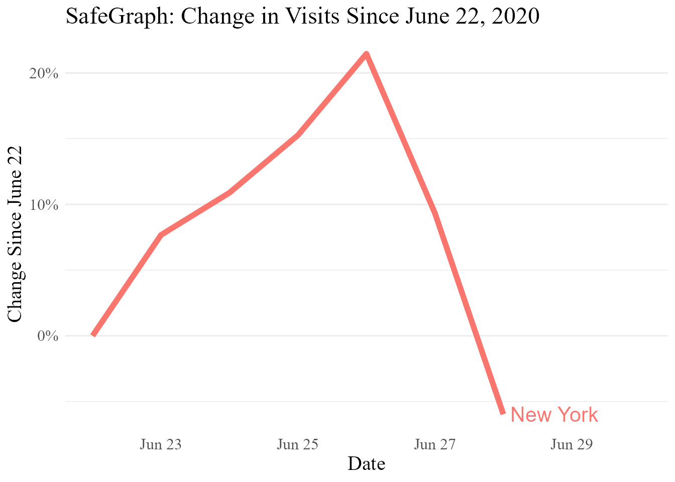
rests <- pat_naics %>%
  # Restaurant codes
  subset(floor(naics_code/1000) == 722)

# The NAICS titles can be too long for graphs, so we won't use naics_codes
short_names <- data.frame(naics_title = unique(rests$naics_title),
                          naics_short = c('Caterer',
                                          'Bar',
                                          'Restaurant',
                                          'Fast Food',
                                          'Cafeteria',
                                          'Cafe'))

rests <- rests %>%
  subset(date == max(pat_naics$date)) %>%
  merge(short_names, by = 'naics_title')
data.table::setorder(rests, -norm_visits)
rests$naics_short <- factor(rests$naics_short, levels = unique(rests$naics_short))

ggplot2::ggplot(rests,ggplot2::aes(x = naics_short, y = norm_visits, fill = norm_visits > 0)) +
  ggplot2::geom_col() +
  ggplot2::geom_text(ggplot2::aes(label = paste(naics_short, scales::percent(norm_visits, accuracy = .1)),
                                  y = norm_visits + .01 - .02*(norm_visits < 0))) +
  ggplot2::theme_minimal() +
  ggplot2::theme(text = ggplot2::element_text(size = 14),
                 plot.title = ggplot2::element_text(size = 14),
                 panel.grid = ggplot2::element_blank()) +
  ggplot2::guides(fill = FALSE) +
  ggplot2::scale_y_continuous(labels = scales::percent) +
  ggplot2::scale_x_discrete(labels = NULL) +
  ggplot2::scale_fill_manual(values = c('#CC0000','black')) +
  ggplot2::labs(x = '', y = 'Change from June 22 to June 29', title = 'SafeGraph: One-Week Change in Visits for Prepared Food Locations')
#> Warning: `guides(<scale> = FALSE)` is deprecated. Please use `guides(<scale> =
#> "none")` instead.